K-Nearest Neighbours(K-NN) algorithm from scratch with a hands-on example (in R)

Part A: K-NN Algorithm from scratch

An Introduction:

Classification algorithms have developed over time from basic models to complex ones providing much more flexibility in dealing with the data and increasing the accuracy. K Nearest Neighbours algorithm is one of the simple, easy to understand and topmost machine learning algorithms (not model) that has its applications in different branches. For example,

Finance: in predicting the credit rating of customers, targeted marketing, loan default prediction and so on
Healthcare: in classifying gene expression
Political Science: classifying voters
Image, video, pattern recognition and so on

If you are well acquainted with the basics of machine learning you can skip this part:

Few important things to know before we begin:

What is the test and train Data?
- In machine learning algorithm we split the dataset in a certain ratio (like a train:test::80:20) and build the model on train dataset. The test dataset is used to evaluate the model efficiency.
What is classification Algorithm?
- Classification is the process of predicting the class of given data points. In layman terms suppose, you have a dataset containing a customers age, gender, location, educational qualification and Magazine X subscription. Now it might be a case where the Magazine X company might want to build a model to categorize the potential market (whether a person will subscribe for the magazine or not?) based on the data available (using age, gender, location, educational qualification).

What are Lazy Learners and Eager Learners?
- Lazy learners simply store the training data and wait until testing data appear. When it does, classification is conducted based on the most related data in the stored training data. Compared to eager learners, lazy learners have less training time but more time in predicting. Example: k-nearest neighbour, Case-based reasoning;
- Eager learners construct a classification model based on the given training data before receiving data for classification. It must be able to commit to a single hypothesis that covers the entire instance space. Due to the model construction, eager learners take a long time to train and less time to predict. Example: Decision Tree, Naive Bayes, Artificial Neural Networks;

What are Supervised Learning and Unsupervised Learning?
- In layman terms, if you supervise your machine while building the model it’s supervised learning, if not then it is unsupervised. To be specific in supervised learning you label your data and tell the machine to treat the data as the label says. For example: you have a dataset like c = [45,34,56,34,78,45,65,… ] for the machine these are just numbers but if you program the algorithm to treat those values as age, you are supervising the learning process of your machine.
What are signal and noise?
- In machine learning, one can think of the “signal” as the true underlying pattern that you wish to learn from the data.
- “Noise” on the other hand, refers to the irrelevant information or randomness in a dataset.
What is the goodness of fit?
- The goodness of fit refers to how closely a model’s prediction matches the observed (true) values.

What is overfitting, underfitting and bias-variance trade-off?
- Underfitting occurs when a model is too simple, a smaller number of features or regularized too much, which makes it inflexible in learning from the dataset.
- On the other hand, considering too many features, trying to fit the predictors beyond a certain level might cause overfitting.
- Bias and variance are two forms of prediction error in machine learning. Reducing error from one might increase error from the other. This trade-off between too simple (high bias) vs. too complex (high variance) is a key concept in statistics and machine learning, and one that affects all supervised learning algorithms.

K-NN Classification:

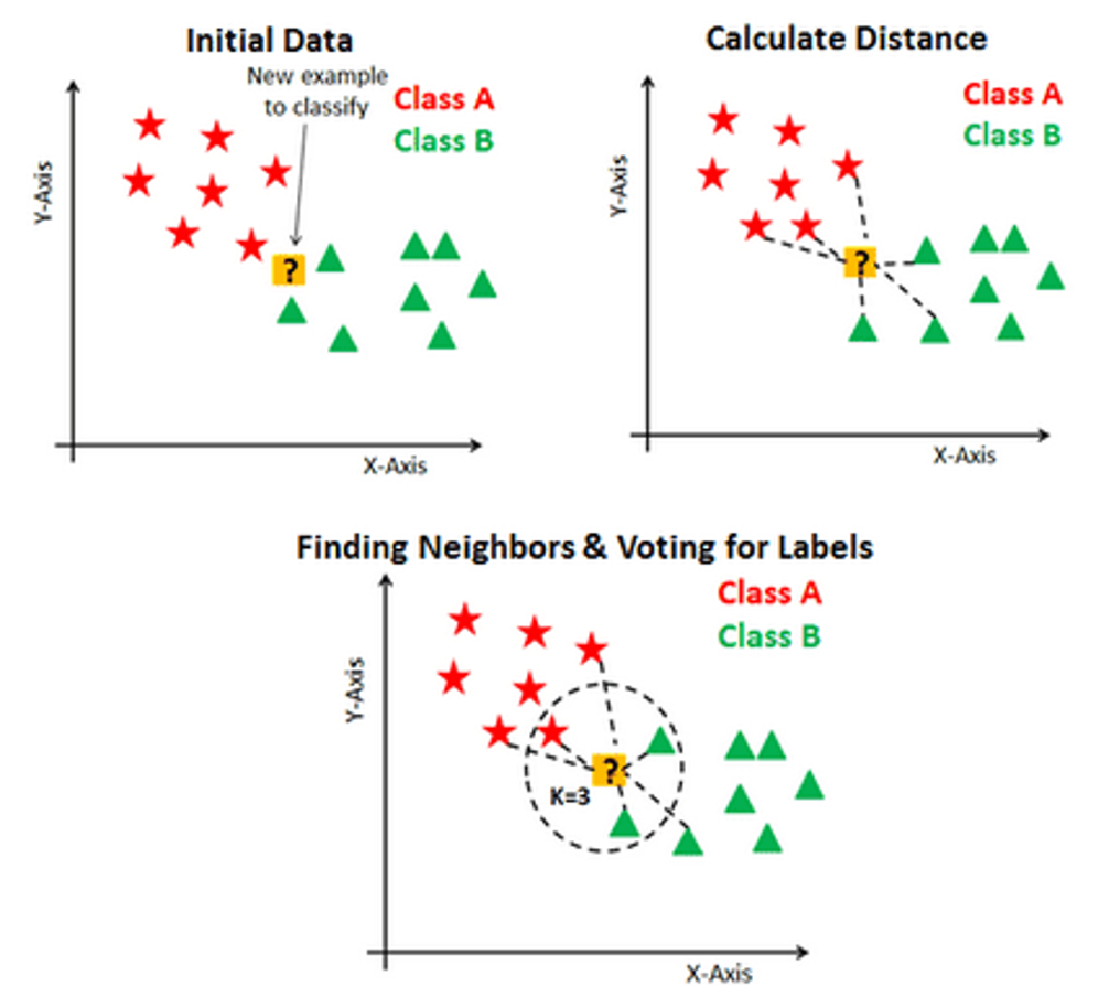
What is k-NN? It is a non-parametric and lazy learning algorithm that stores all the available cases and classifies the new data or case based on a similarity measure. The algorithm assumes that similar things exist in closer proximity.

Assumptions of KNN:

k-NN performs much better if all of the data have the same scale
k-NN works well with a small number of input variables (p) but struggles when the number of inputs is very large
k-NN makes no assumptions about the functional form of the problem is solved

A distance measure is used to assess which of the K instances within the training dataset are most comparable to new input. For real-valued input variables, the most popular distance measure is the Euclidean distance.

Apart from Euclidean distance, there are few other types of measures as well. like-

Manhattan Distance

Chi-Square Distance

Correlation Distance

Hamming Distance

Minkowsky Distance

The K-NN Algorithm:

Load the data
Divide the data into training and test sets
Determine which distance function is to be used
Choose a sample from the test data that needs to be classified and compute the distance to its n training samples
Sort the distances obtained and take the k-nearest data samples
Assign the test class to the class based on the majority vote of its k neighbours.

Performance of the K-NN algorithm is influenced by three main factors:

The distance function or distance matrix used in determining the nearest neighbours.
The decision rule used to derive a classification from the k nearest neighbours.
The number of neighbours(k) used to classify the new data point.

Choosing the right value for k:

To find out the value of K that’s right for the dataset, we need to run the KNN algorithm several times with different values of k and choose the K value that reduces the number of errors we encounter while maintaining the bias-variance trade-off.

Few things to keep in mind while selecting the value of K:

As we decrease the value of K to 1, our predictions become less stable
On the contrary, as we increase the value of K, predictions become more stable due to majority voting, and thus, more likely to make more accurate predictions (up to a certain point). Eventually, we begin to witness an increasing number of errors. It is at this point we know we have pushed the value of K too far.
k should be an odd number to avoid ties.
A conventional way of finding k value is by taking the value Sqrt(n)/2, where n is the total number of data points.
Divide your data into train and tuning (validation) set. Do not use test set for this purpose. Use the validation set to tune your k and find the one that works for your problem.
Elbow method is used to find the value of k in k means algorithms. Do not confuse knn with k means.

Advantages and disadvantages of K-NN Classification:

Advantages	Disadvantages
It is pretty intuitive and simple	Lazy and slow algorithm
Lesser number of assumptions	Curse of Dimensionality
No training step	K-NN needs homogeneous features
It constantly evolves	Highly sensitive to outliers
Single hyper parameter	No capacity for dealing with missing value problems

Part B: Hands-on example of KNN in R

1.Introduction:

Now we are going to perform a hands-on exercise on “Bank Marketing” dataset. (This dataset is publicly available for research. The details are described in [Moro et al., 2011]

[Moro et al., 2011] S. Moro, R. Laureano and P. Cortez. Using Data Mining for Bank Direct Marketing: An Application of the CRISP-DM Methodology.

In P. Novais et al. (Eds.), Proceedings of the European Simulation and Modelling Conference – ESM’2011, pp. 117-121, Guimarães, Portugal, October 2011. EUROSIS.)

2.Data Description:

The dataset contains 17 variables out of which 5 are numeric and rest are categorical. The variables are as follows.

age (numeric)
job : type of job (categorical: “admin.”,”unknown”,”unemployed”,”management”,”housemaid”,”entrepreneur”,”student”,”blue-collar”,”self-employed”,”retired”,”technician”,”services”)
marital : marital status (categorical: “married”,”divorced”,”single”; note: “divorced” means divorced or widowed)
education (categorical: “unknown”,”secondary”,”primary”,”tertiary”)
default: has credit in default? (binary: “yes”,”no”)
balance: average yearly balance, in euros (numeric)
housing: has housing loan? (binary: “yes”,”no”)
loan: has personal loan? (binary: “yes”,”no”),
contact: contact communication type (categorical: “unknown”,”telephone”,”cellular”)
day: last contact day of the month (numeric)
month: last contact month of year (categorical: “jan”, “feb”, “mar”, …, “nov”, “dec”)
duration: last contact duration, in seconds (numeric)
campaign: number of contacts performed during this campaign and for this client (numeric, includes last contact)
pdays: number of days that passed by after the client was last contacted from a previous campaign (numeric, -1 means client was not previously contacted)
previous: number of contacts performed before this campaign and for this client (numeric)
poutcome: outcome of the previous marketing campaign (categorical: “unknown”,”other”,”failure”,”success”)
- Output variable (desired target):
y – has the client subscribed a term deposit? (binary: “yes”,”no”)

Our aim is to build an algorithm to predict whether a person will subscribe to term deposit if age, average yearly balance( in euros), last contact duration( in seconds), number of contacts performed during this campaign and for this client (numeric, includes the last contact) and number of contacts performed before this campaign and for this client (numeric) are provided.

NOTE: Though the K-NN algorithm only considers the numerical characteristics we used this dataset (having only 5 numeric variables) to draw a comparison in the prediction accuracy among different algorithms in upcoming blogs.

3.Loading Libraries:

First, we need to load some libraries.

if(!require(class))install.packages("contrib",repos = "http://cran.us.r-project.org")
if(!require(readr))install.packages("readr",repos = "http://cran.us.r-project.org")
if(!require(knitr))install.packages("knitr",repos = "http://cran.us.r-project.org")
if(!require(tidyverse))install.packages("tidyverse",repos = "http://cran.us.r-project.org")
if(!require(GGally))install.packages("GGally",repos = "http://cran.us.r-project.org")
library(readr)
library(class)
library(tidyverse)
library(GGally)
library(lmtest)

4.Data Analysis:

Loading the dataset

# load the dataset
dataset = read_csv("./Insight/bank_data.csv")

Lets get an idea what we’re working with

#Data Description
MissingValue = sum(which(is.na(dataset)))
MissingValue
head(dataset)
tail(dataset)
summary(dataset)
str(dataset)

age            job              marital           education          default           balance        housing       
 Min.   :18.00   Length:45211       Length:45211       Length:45211       Mode :logical   Min.   : -8019   Mode :logical  
 1st Qu.:33.00   Class :character   Class :character   Class :character   FALSE:44396     1st Qu.:    72   FALSE:20081    
 Median :39.00   Mode  :character   Mode  :character   Mode  :character   TRUE :815       Median :   448   TRUE :25130    
 Mean   :40.94                                                                            Mean   :  1362                  
 3rd Qu.:48.00                                                                            3rd Qu.:  1428                  
 Max.   :95.00                                                                            Max.   :102127
loan           contact               day           month              duration         campaign          pdays      
 Mode :logical   Length:45211       Min.   : 1.00   Length:45211       Min.   :   0.0   Min.   : 1.000   Min.   : -1.0  
 FALSE:37967     Class :character   1st Qu.: 8.00   Class :character   1st Qu.: 103.0   1st Qu.: 1.000   1st Qu.: -1.0  
 TRUE :7244      Mode  :character   Median :16.00   Mode  :character   Median : 180.0   Median : 2.000   Median : -1.0  
                                    Mean   :15.81                      Mean   : 258.2   Mean   : 2.764   Mean   : 40.2  
                                    3rd Qu.:21.00                      3rd Qu.: 319.0   3rd Qu.: 3.000   3rd Qu.: -1.0  
                                    Max.   :31.00                      Max.   :4918.0   Max.   :63.000   Max.   :871.0  
    previous          poutcome             y          
 Min.   :  0.0000   Length:45211       Mode :logical  
 1st Qu.:  0.0000   Class :character   FALSE:39922    
 Median :  0.0000   Mode  :character   TRUE :5289     
 Mean   :  0.5803                                     
 3rd Qu.:  0.0000                                     
 Max.   :275.0000                                     
Classes ‘spec_tbl_df’, ‘tbl_df’, ‘tbl’ and 'data.frame':	45211 obs. of  17 variables:
 $ age      : num  58 44 33 47 33 35 28 42 58 43 ...
 $ job      : chr  "management" "technician" "entrepreneur" "blue-collar" ...
 $ marital  : chr  "married" "single" "married" "married" ...
 $ education: chr  "tertiary" "secondary" "secondary" "unknown" ...
 $ default  : logi  FALSE FALSE FALSE FALSE FALSE FALSE ...
 $ balance  : num  2143 29 2 1506 1 ...
 $ housing  : logi  TRUE TRUE TRUE TRUE FALSE TRUE ...
 $ loan     : logi  FALSE FALSE TRUE FALSE FALSE FALSE ...
 $ contact  : chr  "unknown" "unknown" "unknown" "unknown" ...
 $ day      : num  5 5 5 5 5 5 5 5 5 5 ...
 $ month    : chr  "may" "may" "may" "may" ...
 $ duration : num  261 151 76 92 198 139 217 380 50 55 ...
 $ campaign : num  1 1 1 1 1 1 1 1 1 1 ...
 $ pdays    : num  -1 -1 -1 -1 -1 -1 -1 -1 -1 -1 ...
 $ previous : num  0 0 0 0 0 0 0 0 0 0 ...
 $ poutcome : chr  "unknown" "unknown" "unknown" "unknown" ...
 $ y        : logi  FALSE FALSE FALSE FALSE FALSE FALSE ...

Data visualization

# Histogram Plot of the variables
dataset %>%
  gather(Attribute, Value, c(1)) %>%
  ggplot(aes(x=Value, fill = y)) +
  geom_histogram(color = "black",breaks = seq(0,100,by = 3.5)) +
  theme_bw()+
  labs(x= "Values", y="Frequency",
       title= "Bank Data Set",
       subtitle= "Histogram for age") +
  theme(legend.title = element_blank(),
        legend.position = "bottom")
dataset %>%
  gather(Attribute, Value, c(6)) %>%
  ggplot(aes(x=Value, fill = y)) +
  geom_histogram(color = "black",breaks = seq(-2000,7500,by = 150)) +
  theme_bw()+
  labs(x= "Values", y="Frequency",
       title= "Bank Data Set",
       subtitle= "Histogram for Account balance") +
  theme(legend.title = element_blank(),
        legend.position = "bottom")
dataset %>%
  gather(Attribute, Value, c(13)) %>%
  ggplot(aes(x=Value, fill = y)) +
  geom_histogram(color = "black",breaks = seq(-1,64,by = 1)) +
  theme_bw()+
  labs(x= "Values", y="Frequency",
       title= "Bank Data Set",
       subtitle= "Histogram for number of contacts performed during this campaign and for this client") +
  theme(legend.title = element_blank(),
        legend.position = "bottom")
dataset %>%
  gather(Attribute, Value, c(12)) %>%
  ggplot(aes(x=Value, fill = y)) +
  geom_histogram(color = "black",breaks = seq(0,1000,by = 20)) +
  theme_bw()+
  labs(x= "Values", y="Frequency",
       title= "Bank Data Set",
       subtitle= "Histogram for last contact duration(in sec)") +
  theme(legend.title = element_blank(),
        legend.position = "bottom")
dataset %>%
  gather(Attribute, Value, c(15)) %>%
  ggplot(aes(x=Value, fill = y)) +
  geom_histogram(color = "black",breaks = seq(-1,10,by = 1)) +
  theme_bw()+
  labs(x= "Values", y="Frequency",
       title= "Bank Data Set",
       subtitle= "Histogram for contacts performed before this campaign (-1 value is considered if not contacted previously ") +
  theme(legend.title = element_blank(),
        legend.position = "bottom")

# Density plot for each variable
dataset %>%
  gather(Attributes, value,c(1)) %>%
  ggplot(aes(x=value, fill=y)) +
  geom_density(colour="black", alpha = .5) +
  facet_wrap(~Attributes, scales="free_x") +
  labs(x="Values", y="Density",
       title="Bank dataset",
       subtitle="Density plot for each Variable") +
  theme_bw() +
  theme(legend.position="bottom",
        legend.title=element_blank())
dataset %>%
  gather(Attributes, value,c(6)) %>%
  ggplot(aes(x=value, fill=y)) +
  geom_density(colour="black", alpha = .5) +
  xlim(-1000,10000)+
  facet_wrap(~Attributes, scales="free_x") +
  labs(x="Values", y="Density",
       title="Bank dataset",
       subtitle="Density plot for each Variable") +
  theme_bw() +
  theme(legend.position="bottom",
        legend.title=element_blank())
dataset %>%
  gather(Attributes, value,c(12)) %>%
  ggplot(aes(x=value, fill=y)) +
  geom_density(colour="black", alpha = .5) +
  xlim(0,2000)+
  facet_wrap(~Attributes, scales="free_x") +
  labs(x="Values", y="Density",
       title="Bank dataset",
       subtitle="Density plot for each Variable") +
  theme_bw() +
  theme(legend.position="bottom",
        legend.title=element_blank())
dataset %>%
  gather(Attributes, value,c(13)) %>%
  ggplot(aes(x=value, fill=y)) +
  geom_density(colour="black", alpha = .5) +
  xlim(0,12.5)+
  facet_wrap(~Attributes, scales="free_x") +
  labs(x="Values", y="Density",
       title="Bank dataset",
       subtitle="Density plot for each Variable") +
  theme_bw() +
  theme(legend.position="bottom",
        legend.title=element_blank())

dataset %>%
  gather(Attributes, value,c(15)) %>%
  ggplot(aes(x=value, fill=y)) +
  geom_density(colour="black", alpha = .5) +
  xlim(0,10)+
  facet_wrap(~Attributes, scales="free_x") +
  labs(x="Values", y="Density",
       title="Bank dataset",
       subtitle="Density plot for each Variable") +
  theme_bw() +
  theme(legend.position="bottom",
        legend.title=element_blank())

# Violin plot for each attribute
dataNorm = dataset
dataNorm[,c(1,6,12,13,15)] = scale(dataset[,c(1,6,12,13,15)])
dataNorm %>%
  gather(Attributes, value, c(1,6,12,13,15)) %>%
  ggplot(aes(x=reorder(Attributes, value, FUN=median), y=value, fill=Attributes,)) +
  ylim(-2,3.5)+
  geom_violin(show.legend=FALSE) +
  labs(title="Bank dataset",
       subtitle="Violin plot for each attribute") +
  theme_bw() +
  theme(axis.title.y=element_blank(),
        axis.title.x=element_blank())

# Scatter plot and correlations
ggpairs(cbind(dataNorm, Cluster=as.factor(dataNorm$y)),
        columns = c(1,6,12,13,15), aes(colour=Cluster, alpha=0.5),
        lower=list(continuous="points"),
        axisLabels="none", switch="both") +
        theme_bw()

5.Data Preparation:

# Data Preparation
dataset2 = dataNorm
dataset2[,c(2,3,4,5,7,8,9,10,11,14,16,17)] = lapply(dataNorm[,c(2,3,4,5,7,8,9,10,11,14,16,17)],factor)
sapply(dataset2,class)

Test-train split

# test-train split
set.seed(1000)
num = sample(2,nrow(dataset2),replace = TRUE,prob = c(0.8,0.2))
trainData = dataset2[num == 1,]
testData = dataset2[num == 2,]
trainData2 = trainData[,c(1,6,12,13,15,17)]
testData2 = testData[,c(1,6,12,13,15,17)]

6.K-NN Execution:

The knn() function has the following main arguments:

train. Matrix or data frame of training set cases.
test. Matrix or data frame of test set cases. A vector will be interpreted as a row vector for a single case.
cl. Factor of true classifications of the training set.
k. The number of neighbours considered.

#k-NN with k=1
KnnPrediction_k1 = knn(trainData2[,-6], testData2[,-6],factor(trainData$y), k=1)

#k-NN with k=2
KnnPrediction_k2 = knn(trainData2[,-6], testData2[,-6],factor(trainData$y), k=2)

#k-NN with k3=
KnnPrediction_k3 = knn(trainData2[,-6], testData2[,-6],factor(trainData$y), k=3)

#k-NN with k=4
KnnPrediction_k4 = knn(trainData2[,-6], testData2[,-6],factor(trainData$y), k=4)

#k-NN with k=sqrt(N)/2; where N =  no of observations
KnnPrediction_ksqrtn = knn(trainData2[,-6], testData2[,-6],factor(trainData$y), k=((length(trainData2))^.5/2))

table(testData$y, KnnPrediction_k1)
# Classification accuracy of KnnTestPrediction_k1
sum(KnnPrediction_k1==testData$y)/length(testData$y)*100

table(testData$y, KnnPrediction_k2)
# Classification accuracy of KnnTestPrediction_k2
sum(KnnPrediction_k2==testData$y)/length(testData$y)*100

table(testData$y, KnnPrediction_k3)
# Classification accuracy of KnnTestPrediction_k1
sum(KnnPrediction_k3==testData$y)/length(testData$y)*100

table(testData$y, KnnPrediction_k4)
# Classification accuracy of KnnTestPrediction_k1
sum(KnnPrediction_k4==testData$y)/length(testData$y)*100

table(testData$y, KnnPrediction_ksqrtn)
# Classification accuracy of KnnTestPrediction_k1
sum(KnnPrediction_ksqrtn==testData$y)/length(testData$y)*100

Confusion Matrix with accuracy-

   KnnPrediction_k1
        FALSE TRUE
  FALSE  7244  640
  TRUE    734  365
[1] 84.70444
       KnnPrediction_k2
        FALSE TRUE
  FALSE  7220  664
  TRUE    743  356
[1] 84.33708
       KnnPrediction_k3
        FALSE TRUE
  FALSE  7517  367
  TRUE    787  312
[1] 87.15351
       KnnPrediction_k4
        FALSE TRUE
  FALSE  7518  366
  TRUE    775  324
[1] 87.29823
       KnnPrediction_ksqrtn
        FALSE TRUE
  FALSE  7244  640
  TRUE    734  365
[1] 84.70444

7.Evaluation:

With different values of k, we can use the confusion matrix to test the accuracy of previous classifications and study which one offers the best results.To study graphically which value of k gives us the best classification, we can plot Accuracy vs Choice of k.

#accuracy vs choice of K
KnnPrediction = list()
accuracy = numeric()
for (k in 1: 100){
  KnnPrediction[[k]] = knn(trainData2[,-6],
                           testData2[,-6],factor(trainData$y), k, prob = TRUE)
  accuracy[k] = sum(KnnPrediction[[k]]==testData2$y)/length(testData2$y)*100
}

plot(accuracy, type = "b" , col = "light green",cex = 1, pch = 20,
     xlab = "k(Number Of Neighbours)",ylab = "Classification accuracy( in %)",
     main = "Accuracy vs Number of Neighbours")
abline(v=which(accuracy==max(accuracy)), col = "red", lwd = 1.5)
abline(h=max(accuracy), col = "light blue", lty = 3)
abline(h=min(accuracy), col = "light blue", lty = 3)

From the plot we can see that for the value of k = 65 maximum accuracy classification algorithm is achived (~89%). So in this case for further classification we will use k value 65.

8.Summary:

Finally we are at the end, in this discussion, we have learned about the K-Nearest Neighbour Algorithm, including the data preparation (normalization and division in two parts) and the evaluation part as well. Hope you found it helpful!! The complete code is given below.

# loading required packages
if(!require(class))install.packages("contrib",repos = "http://cran.us.r-project.org")
if(!require(readr))install.packages("readr",repos = "http://cran.us.r-project.org")
if(!require(knitr))install.packages("knitr",repos = "http://cran.us.r-project.org")
if(!require(tidyverse))install.packages("tidyverse",repos = "http://cran.us.r-project.org")
if(!require(GGally))install.packages("GGally",repos = "http://cran.us.r-project.org")
if(!require(animation))install.packages("animation",repos = "http://cran.us.r-project.org")
library(animation)
library(readr)
library(class)
library(tidyverse)
library(GGally)
library(lmtest)

# load the dataset
dataset = read_csv("C:/Users/Neeladri Shekhar Pal/Desktop/Insight/bank_data.csv")

#Data Description
MissingValue = sum(which(is.na(dataset)))
MissingValue
head(dataset)
tail(dataset)
summary(dataset)
str(dataset)

# Data Analysis
dataset %>%
  gather(Attribute, Value, c(1)) %>%
  ggplot(aes(x=Value, fill = y)) +
  geom_histogram(color = "black",breaks = seq(0,100,by = 3.5)) +
  theme_bw()+
  labs(x= "Values", y="Frequency",
       title= "Bank Data Set",
       subtitle= "Histogram for age") +
  theme(legend.title = element_blank(),
        legend.position = "bottom")
dataset %>%
  gather(Attribute, Value, c(6)) %>%
  ggplot(aes(x=Value, fill = y)) +
  geom_histogram(color = "black",breaks = seq(-2000,7500,by = 150)) +
  theme_bw()+
  labs(x= "Values", y="Frequency",
       title= "Bank Data Set",
       subtitle= "Histogram for Account balance") +
  theme(legend.title = element_blank(),
        legend.position = "bottom")
dataset %>%
  gather(Attribute, Value, c(13)) %>%
  ggplot(aes(x=Value, fill = y)) +
  geom_histogram(color = "black",breaks = seq(-1,64,by = 1)) +
  theme_bw()+
  labs(x= "Values", y="Frequency",
       title= "Bank Data Set",
       subtitle= "Histogram for number of contacts performed during this campaign and for this client") +
  theme(legend.title = element_blank(),
        legend.position = "bottom")
dataset %>%
  gather(Attribute, Value, c(12)) %>%
  ggplot(aes(x=Value, fill = y)) +
  geom_histogram(color = "black",breaks = seq(0,1000,by = 20)) +
  theme_bw()+
  labs(x= "Values", y="Frequency",
       title= "Bank Data Set",
       subtitle= "Histogram for last contact duration(in sec)") +
  theme(legend.title = element_blank(),
        legend.position = "bottom")
dataset %>%
  gather(Attribute, Value, c(15)) %>%
  ggplot(aes(x=Value, fill = y)) +
  geom_histogram(color = "black",breaks = seq(-1,10,by = 1)) +
  theme_bw()+
  labs(x= "Values", y="Frequency",
       title= "Bank Data Set",
       subtitle= "Histogram for contacts performed before this campaign (-1 value is considered if not contacted previously ") +
  theme(legend.title = element_blank(),
        legend.position = "bottom")

# Density plot for each variable
dataset %>%
  gather(Attributes, value,c(1)) %>%
  ggplot(aes(x=value, fill=y)) +
  geom_density(colour="black", alpha = .5) +
  facet_wrap(~Attributes, scales="free_x") +
  labs(x="Values", y="Density",
       title="Bank dataset",
       subtitle="Density plot for each Variable") +
  theme_bw() +
  theme(legend.position="bottom",
        legend.title=element_blank())
dataset %>%
  gather(Attributes, value,c(6)) %>%
  ggplot(aes(x=value, fill=y)) +
  geom_density(colour="black", alpha = .5) +
  xlim(-1000,10000)+
  facet_wrap(~Attributes, scales="free_x") +
  labs(x="Values", y="Density",
       title="Bank dataset",
       subtitle="Density plot for each Variable") +
  theme_bw() +
  theme(legend.position="bottom",
        legend.title=element_blank())
dataset %>%
  gather(Attributes, value,c(12)) %>%
  ggplot(aes(x=value, fill=y)) +
  geom_density(colour="black", alpha = .5) +
  xlim(0,2000)+
  facet_wrap(~Attributes, scales="free_x") +
  labs(x="Values", y="Density",
       title="Bank dataset",
       subtitle="Density plot for each Variable") +
  theme_bw() +
  theme(legend.position="bottom",
        legend.title=element_blank())
dataset %>%
  gather(Attributes, value,c(13)) %>%
  ggplot(aes(x=value, fill=y)) +
  geom_density(colour="black", alpha = .5) +
  xlim(0,12.5)+
  facet_wrap(~Attributes, scales="free_x") +
  labs(x="Values", y="Density",
       title="Bank dataset",
       subtitle="Density plot for each Variable") +
  theme_bw() +
  theme(legend.position="bottom",
        legend.title=element_blank())

dataset %>%
  gather(Attributes, value,c(15)) %>%
  ggplot(aes(x=value, fill=y)) +
  geom_density(colour="black", alpha = .5) +
  xlim(0,10)+
  facet_wrap(~Attributes, scales="free_x") +
  labs(x="Values", y="Density",
       title="Bank dataset",
       subtitle="Density plot for each Variable") +
  theme_bw() +
  theme(legend.position="bottom",
        legend.title=element_blank())

# Violin plot for each attribute
dataNorm = dataset
dataNorm[,c(1,6,12,13,15)] = scale(dataset[,c(1,6,12,13,15)])
dataNorm %>%
  gather(Attributes, value, c(1,6,12,13,15)) %>%
  ggplot(aes(x=reorder(Attributes, value, FUN=median), y=value, fill=Attributes,)) +
  ylim(-2,3.5)+
  geom_violin(show.legend=FALSE) +
  labs(title="Bank dataset",
       subtitle="Violin plot for each attribute") +
  theme_bw() +
  theme(axis.title.y=element_blank(),
        axis.title.x=element_blank())

# Scatter plot and correlations
ggpairs(cbind(dataNorm, Cluster=as.factor(dataNorm$y)),
        columns = c(1,6,12,13,15), aes(colour=Cluster, alpha=0.5),
        lower=list(continuous="points"),
        axisLabels="none", switch="both") +
  theme_bw()

# Data Preparation
dataset2 = dataNorm
dataset2[,c(2,3,4,5,7,8,9,10,11,14,16,17)] = lapply(dataNorm[,c(2,3,4,5,7,8,9,10,11,14,16,17)],factor)
sapply(dataset2,class)

# test-train split
set.seed(1000)
num = sample(2,nrow(dataset2),replace = TRUE,prob = c(0.8,0.2))
trainData = dataset2[num == 1,]
testData = dataset2[num == 2,]
trainData2 = trainData[,c(1,6,12,13,15,17)]
testData2 = testData[,c(1,6,12,13,15,17)]
summary(testData)
head(testData)

#
#k-NN with k=1
KnnPrediction_k1 = knn(trainData2[,-6], testData2[,-6],factor(trainData$y), k=1)

#k-NN with k=2
KnnPrediction_k2 = knn(trainData2[,-6], testData2[,-6],factor(trainData$y), k=2)

#k-NN with k3=
KnnPrediction_k3 = knn(trainData2[,-6], testData2[,-6],factor(trainData$y), k=3)

#k-NN with k=4
KnnPrediction_k4 = knn(trainData2[,-6], testData2[,-6],factor(trainData$y), k=4)

#k-NN with k=sqrt(N)/2; where N =  no of observations
KnnPrediction_ksqrtn = knn(trainData2[,-6], testData2[,-6],factor(trainData$y), k=((length(trainData2))^.5/2))

table(testData$y, KnnPrediction_k1)
# Classification accuracy of KnnTestPrediction_k1
sum(KnnPrediction_k1==testData$y)/length(testData$y)*100

table(testData$y, KnnPrediction_k2)
# Classification accuracy of KnnTestPrediction_k2
sum(KnnPrediction_k2==testData$y)/length(testData$y)*100

table(testData$y, KnnPrediction_k3)
# Classification accuracy of KnnTestPrediction_k1
sum(KnnPrediction_k3==testData$y)/length(testData$y)*100

table(testData$y, KnnPrediction_k4)
# Classification accuracy of KnnTestPrediction_k1
sum(KnnPrediction_k4==testData$y)/length(testData$y)*100

table(testData$y, KnnPrediction_ksqrtn)
# Classification accuracy of KnnTestPrediction_k1
sum(KnnPrediction_ksqrtn==testData$y)/length(testData$y)*100

#accuracy vs choice of K
KnnPrediction = list()
accuracy = numeric()
for (k in 1: 100){
  KnnPrediction[[k]] = knn(trainData2[,-6],
                           testData2[,-6],factor(trainData$y), k, prob = TRUE)
  accuracy[k] = sum(KnnPrediction[[k]]==testData2$y)/length(testData2$y)*100
}

plot(accuracy, type = "b" , col = "light green",cex = 1, pch = 20,
     xlab = "k(Number Of Neighbours)",ylab = "Classification accuracy( in %)",
     main = "Accuracy vs Number of Neighbours")
abline(v=which(accuracy==max(accuracy)), col = "red", lwd = 1.5)
abline(h=max(accuracy), col = "light blue", lty = 3)
abline(h=min(accuracy), col = "light blue", lty = 3)